# -*- coding: utf-8 -*
from sklearn.datasets import load_digits
from sklearn.cluster import KMeans
import matplotlib.pyplot as plt
from scipy.stats import mode
import numpy as np
from sklearn.metrics import accuracy_score
from sklearn.metrics import confusion_matrix
import seaborn as sns
from sklearn.manifold import TSNE  # 非线性嵌入算法模块

digits = load_digits()
# print(digits.data.shape)
kmeans = KMeans(n_clusters=10, random_state=0)
clusters = kmeans.fit_predict(digits.data)
# print(kmeans.cluster_centers_.shape)

fig, ax = plt.subplots(2, 5, figsize=(8, 3))
centers = kmeans.cluster_centers_.reshape(10, 8, 8)
for axi, center in zip(ax.flat, centers):
    axi.set(xticks=[], yticks=[])
    axi.imshow(center, interpolation='nearest', cmap=plt.cm.binary)

labels = np.zeros_like(clusters)  # 建立类似clusters的全0数组
# print('clusters:\n', clusters)
# print('clusters.shape:\n', clusters.shape)
# print('labels:\n', labels)
for i in range(10):  # 纠正labels,让每个簇估计出的数字服从出现最大概率的数字
    mask = (clusters == i)  # 对于等于某个数字的簇形成的mask
    # print('mask:\n', mask)
    # print('digits.target[mask]:\n', digits.target[mask])  # 筛选出mask罩出的判断值
    # 用mask选出并纠正labels里每个簇里的各个值,化为target里被mask罩出(估计)的大多数值一样
    labels[mask] = mode(digits.target[mask])[0]  # mode(): 返回传入数组/矩阵中最常出现的成员以及出现的次数,如果多个成员出现次数一样多,返回值小的那个
    # print('labels[mask]:\n', labels[mask])  # 改变后
print('accuracy_score is: ', accuracy_score(digits.target, labels))
fig2, ax2 = plt.subplots()
mat = confusion_matrix(digits.target, labels)
sns.heatmap(mat.T, square=True, annot=True, fmt='d', cbar=False, xticklabels=digits.target_names,
            yticklabels=digits.target_names)
plt.xlabel('true label')
plt.ylabel('predicted label')

# 预处理,投影数据到二维
# 初始化,默认为random。取值为random为随机初始化,取值为pca为利用PCA进行初始化(常用),取值为numpy数组时必须shape=(n_samples, n_components)
tsne = TSNE(n_components=2, init='pca', random_state=0)
digits_proj = tsne.fit_transform(digits.data)
# 计算簇
kmeans = KMeans(n_clusters=10, random_state=0)
clusters = kmeans.fit_predict(digits_proj)
# 对应统一标签
labels = np.zeros_like(clusters)
for i in range(10):
    mask = (clusters == i)
    labels[mask] = mode(digits.target[mask])[0]
print('accuracy_score is: ', accuracy_score(digits.target, labels))
plt.show()
PCA特征脸
# -*- coding: UTF-8 -*-
import numpy as np
import matplotlib.pyplot as plt
import seaborn
from sklearn.datasets import fetch_lfw_people
from sklearn.decomposition import PCA
seaborn.set()

faces = fetch_lfw_people(min_faces_per_person=60)
print(faces.target_names)
print(faces.images.shape)  # 1348张图片,62*47矩阵供显示
print(faces.data.shape)  # 1348张图,每张图2914特征维度
pca = PCA(150)  # 随机前150个主成分
pca.fit(faces.data)
fig, axes = plt.subplots(3, 8, figsize=(9, 4), subplot_kw={'xticks': [], 'yticks': []},
                         gridspec_kw=dict(hspace=0.1, wspace=0.1))
for i, ax in enumerate(axes.flat):
    ax.imshow(pca.components_[i].reshape(62, 47), cmap='bone')  # 展示每个特诊维度的综合画像
print('pca.components_:\n', pca.components_.shape)  # 150个特征,2914张照片
fig2 = plt.figure()
plt.plot(np.cumsum(pca.explained_variance_ratio_))
plt.xlabel('number of components')
plt.ylabel('cumulative explained variance')

pca = PCA(150).fit(faces.data)
components = pca.transform(faces.data)
projected = pca.inverse_transform(components)
fig, ax = plt.subplots(2, 10, figsize=(10, 2.5),
                       subplot_kw={'xticks': [], 'yticks': []},
                       gridspec_kw=dict(hspace=0.1, wspace=0.1))
for i in range(10):
    ax[0, i].imshow(faces.data[i].reshape(62, 47), cmap='binary_r')
    ax[1, i].imshow(projected[i].reshape(62, 47), cmap='binary_r')
ax[0, 0].set_ylabel('full-dim\ninput')
ax[1, 0].set_ylabel('150-dim\nreconstruction')
plt.show()
k最近邻算法引用
# -*- coding: utf-8 -*-
import matplotlib.pyplot as plt
import seaborn as sns
import numpy as np
from sklearn.datasets.samples_generator import make_blobs
from sklearn.cluster import KMeans

sns.set()
X, y_true = make_blobs(n_samples=300, centers=4,
                       cluster_std=0.60, random_state=0)
# plt.scatter(X[:, 0], X[:, 1], s=50)
kmeans = KMeans(n_clusters=4)
kmeans.fit(X)
y_kmeans = kmeans.predict(X)  # 返回颜色信息列表
# print('y_kmeans:\n', y_kmeans)
plt.scatter(X[:, 0], X[:, 1], c=y_kmeans, s=50, cmap='viridis')
centers = kmeans.cluster_centers_
print('centers:\n', centers)
plt.scatter(centers[:, 0], centers[:, 1], c='black', s=200, alpha=0.5)

plt.show()
k最近邻算法实现
# -*- coding: utf-8 -*-
import matplotlib.pyplot as plt
import seaborn as sns
import numpy as np
from sklearn.datasets.samples_generator import make_blobs
from sklearn.metrics import pairwise_distances_argmin
sns.set()


def find_clusters(X, n_clusters, rseed=2):
    rng = np.random.RandomState(rseed)
    # 随机选择簇中心点
    print('rng.permutation(X.shape[0])[:n_clusters]:\n', rng.permutation(X.shape[0])[:n_clusters])
    i = rng.permutation(X.shape[0])[:n_clusters]  # 随机排序X.shape[0](300个点,取出前nclusters个)
    centers = X[i]  # 随机选出这四个点坐标
    print('centers:\n', centers)
    while True:  # 一直执行
        # 基于最近中心指定标签
        labels = pairwise_distances_argmin(X, centers)
        # print('labels= ', labels)  # 是一个表示分类的列表
        # 根据各个分类里的点平均值找到新的中心
        new_centers = np.array([X[labels == i].mean(0) for i in range(n_clusters)])  # .mean(0)跨行求平均
        # print('new_centers:\n', new_centers)
        if np.all(centers == new_centers):
            break
        centers = new_centers
    return centers, labels


X, y_true = make_blobs(n_samples=300, centers=4, cluster_std=0.60, random_state=0)
centers, labels = find_clusters(X, 4)
plt.scatter(X[:, 0], X[:, 1], c=labels,
            s=50, cmap='viridis')
plt.show()
矩阵坐标的指定
# -*- coding: utf-8 -*-
import numpy as np
data = np.array([[1, 2, 3],
                 [4, 5, 6],
                 [7, 8, 9]])
i = [0, 1, 2]
j = np.array([2, 1, 0])
print('data[i, j]:\n', data[i, j]) # 指定矩阵的坐标的时候,记住需要是numpy的array而不是python自己的列表格式
高斯基函数的正则化
# -*- coding: UTF-8 -*-
from sklearn.pipeline import make_pipeline
import numpy as np
from sklearn.linear_model import LinearRegression
import matplotlib.pyplot as plt
from sklearn.base import BaseEstimator, TransformerMixin  # 估算器,转换器
from sklearn.linear_model import Ridge
from sklearn.linear_model import Lasso


class GaussianFeatures(BaseEstimator, TransformerMixin):

    def __init__(self, N, width_factor=2.0):
        self.N = N
        self.width_factor = width_factor

    @staticmethod  # 调用静态方法,可以不实例化
    def _gauss_basis(x, y, width, axis=None):
        arg = (x - y) / width
        print('x:\n', x)
        print('y:\n', y)
        print('width:\n', width)
        print('arg = (x - y) / width:\n', ((x - y) / width))
        print('np.exp(-0.5 * np.sum(arg ** 2, axis)).shape: ', np.exp(-0.5 * np.sum(arg ** 2, axis)).shape)
        return np.exp(-0.5 * np.sum(arg ** 2, axis))  # 列向求和

    def fit(self, X, y=None):  # 学习部分
        # 在数据区间内创建N个高斯分布中心
        self.centers_ = np.linspace(X.min(), X.max(), self.N)  # 沿x轴均分点形成的数组
        self.width_ = self.width_factor * (self.centers_[1] - self.centers_[0])  # 沿x轴均分点的间距*宽度系数
        # print('self.width_:', self.width_)
        return self  # 返回类对象自己

    def transform(self, X):  # 预测部分
        print('transform.shape: ', self._gauss_basis(X[:, :, np.newaxis], self.centers_,
                                 self.width_, axis=1).shape)
        return self._gauss_basis(X[:, :, np.newaxis], self.centers_,
                                 self.width_, axis=1)  # 列向


rng = np.random.RandomState(1)
x = 10 * rng.rand(50)  # 制作50个随机数
y = np.sin(x) + 0.1 * rng.randn(50)  # 目标数组
xfit = np.linspace(0, 10, 1000)  # 用做预测的数据
'''
# 预定义模型
gauss_model = make_pipeline(GaussianFeatures(20),
                            LinearRegression())
print('=========================================================')
gauss_model.fit(x[:, np.newaxis], y)  # 代入转置后的x矩阵进行学习
print('---------------------------------------------------------')
yfit = gauss_model.predict(xfit[:, np.newaxis])  # 预测结果,得到y值
print('=========================================================')
print('yfit.shape:', yfit.shape)
plt.scatter(x, y)  # 学习数据
plt.plot(xfit, yfit)  # 预测效果曲线
plt.xlim(0, 10)
'''


def basis_plot(model, title=None):
    fig, ax = plt.subplots(2, sharex=True)
    model.fit(x[:, np.newaxis], y)
    ax[0].scatter(x, y)
    ax[0].plot(xfit, model.predict(xfit[:, np.newaxis]))
    ax[0].set(xlabel='x', ylabel='y', ylim=(-1.5, 1.5))

    if title:
        ax[0].set_title(title)

    ax[1].plot(model.steps[0][1].centers_,  # model.steps[0][1] 按步骤定位到GaussianFeatures对象
               model.steps[1][1].coef_)  # model.steps[1][1] 按步骤定位到ridge对象
    print('model.steps[0][1].centers_,: \n', model.steps[0][1])
    print('model.steps[1][1].coef_: \n', model.steps[1][1])
    ax[1].set(xlabel='basis location',
              ylabel='coefficient',
              xlim=(0, 10))


# model = make_pipeline(GaussianFeatures(30), LinearRegression())
# basis_plot(model)
# model = make_pipeline(GaussianFeatures(30), Ridge(alpha=0.1))  # 用带正则化的岭回归
# basis_plot(model, title='Ridge Regression')
model = make_pipeline(GaussianFeatures(30), Lasso(alpha=0.001))
basis_plot(model, title='Lasso Regression')
plt.show()
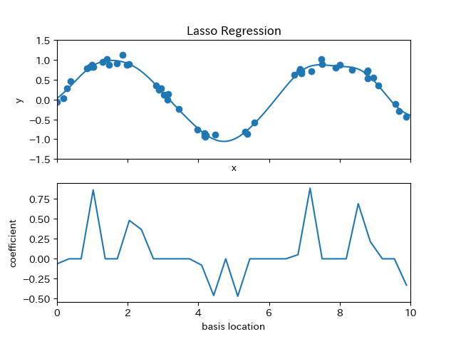
lasso更倾向于把系数设为0, 系数越高表示越过拟合
高斯基函数拟合正弦曲线
# -*- coding: UTF-8 -*-
from sklearn.pipeline import make_pipeline
import numpy as np
from sklearn.linear_model import LinearRegression
import matplotlib.pyplot as plt
from sklearn.base import BaseEstimator, TransformerMixin  # 估算器,转换器


class GaussianFeatures(BaseEstimator, TransformerMixin):

    def __init__(self, N, width_factor=2.0):
        self.N = N
        self.width_factor = width_factor

    @staticmethod  # 调用静态方法,可以不实例化
    def _gauss_basis(x, y, width, axis=None):
        arg = (x - y) / width
        print('x:\n', x)
        print('y:\n', y)
        print('width:\n', width)
        print('arg = (x - y) / width:\n', ((x - y) / width))
        print('np.exp(-0.5 * np.sum(arg ** 2, axis)).shape: ', np.exp(-0.5 * np.sum(arg ** 2, axis)).shape)
        return np.exp(-0.5 * np.sum(arg ** 2, axis))  # 列向求和

    def fit(self, X, y=None):  # 学习部分
        # 在数据区间内创建N个高斯分布中心
        self.centers_ = np.linspace(X.min(), X.max(), self.N)  # 沿x轴均分点形成的数组
        self.width_ = self.width_factor * (self.centers_[1] - self.centers_[0])  # 沿x轴均分点的间距*宽度系数
        # print('self.width_:', self.width_)
        return self  # 返回类对象自己

    def transform(self, X):  # 预测部分
        return self._gauss_basis(X[:, :, np.newaxis], self.centers_,
                                 self.width_, axis=1)  # 列向


# 预定义模型
gauss_model = make_pipeline(GaussianFeatures(20),
                            LinearRegression())
rng = np.random.RandomState(1)
x = 10 * rng.rand(50)  # 制作50个随机数
y = np.sin(x) + 0.1 * rng.randn(50)  # 目标数组
print('=========================================================')
gauss_model.fit(x[:, np.newaxis], y)  # 代入转置后的x矩阵进行学习
xfit = np.linspace(0, 10, 1000)  # 用做预测的数据
print('---------------------------------------------------------')
yfit = gauss_model.predict(xfit[:, np.newaxis])  # 预测结果,得到y值
print('=========================================================')
print('yfit.shape:', yfit.shape)
plt.scatter(x, y)  # 学习数据
plt.plot(xfit, yfit)  # 预测效果曲线
plt.xlim(0, 10)
plt.show()
高斯基底函数参照:
https://gihyo.jp/assets/images/dev/serial/01/machine-learning/0009/002.png
装饰器的运用示例
# -*- coding: UTF-8 -*-


def log(func):
    def wrapper(*arg, **kw):
        print('Start %s: ' % func)
        print('arg: ', arg)
        print('*arg: ', *arg)
        print('kw: ', kw)
        print('*kw: ', *kw)
        return func(*arg, **kw)
    return wrapper


@log  # 用上log装饰器
def func_a(*arg, **kw):
    print('------------------')
    print('ongoing func_a')


def func_b(*arg, **kw):
    print('------------------')
    print('ongoing func_b')


func_a(1, 2, 3, 5, 6, 7, a=1, b=2)
func_b(1, 2, 3, 5, 6, 7, a=1, b=2)
