高斯基函数的正则化

# -*- coding: UTF-8 -*-
from sklearn.pipeline import make_pipeline
import numpy as np
from sklearn.linear_model import LinearRegression
import matplotlib.pyplot as plt
from sklearn.base import BaseEstimator, TransformerMixin  # 估算器，转换器
from sklearn.linear_model import Ridge
from sklearn.linear_model import Lasso


class GaussianFeatures(BaseEstimator, TransformerMixin):

    def __init__(self, N, width_factor=2.0):
        self.N = N
        self.width_factor = width_factor

    @staticmethod  # 调用静态方法，可以不实例化
    def _gauss_basis(x, y, width, axis=None):
        arg = (x - y) / width
        print('x:\n', x)
        print('y:\n', y)
        print('width:\n', width)
        print('arg = (x - y) / width:\n', ((x - y) / width))
        print('np.exp(-0.5 * np.sum(arg ** 2, axis)).shape: ', np.exp(-0.5 * np.sum(arg ** 2, axis)).shape)
        return np.exp(-0.5 * np.sum(arg ** 2, axis))  # 列向求和

    def fit(self, X, y=None):  # 学习部分
        # 在数据区间内创建N个高斯分布中心
        self.centers_ = np.linspace(X.min(), X.max(), self.N)  # 沿x轴均分点形成的数组
        self.width_ = self.width_factor * (self.centers_[1] - self.centers_[0])  # 沿x轴均分点的间距*宽度系数
        # print('self.width_:', self.width_)
        return self  # 返回类对象自己

    def transform(self, X):  # 预测部分
        print('transform.shape: ', self._gauss_basis(X[:, :, np.newaxis], self.centers_,
                                 self.width_, axis=1).shape)
        return self._gauss_basis(X[:, :, np.newaxis], self.centers_,
                                 self.width_, axis=1)  # 列向


rng = np.random.RandomState(1)
x = 10 * rng.rand(50)  # 制作50个随机数
y = np.sin(x) + 0.1 * rng.randn(50)  # 目标数组
xfit = np.linspace(0, 10, 1000)  # 用做预测的数据
'''
# 预定义模型
gauss_model = make_pipeline(GaussianFeatures(20),
                            LinearRegression())
print('=========================================================')
gauss_model.fit(x[:, np.newaxis], y)  # 代入转置后的x矩阵进行学习
print('---------------------------------------------------------')
yfit = gauss_model.predict(xfit[:, np.newaxis])  # 预测结果，得到y值
print('=========================================================')
print('yfit.shape:', yfit.shape)
plt.scatter(x, y)  # 学习数据
plt.plot(xfit, yfit)  # 预测效果曲线
plt.xlim(0, 10)
'''


def basis_plot(model, title=None):
    fig, ax = plt.subplots(2, sharex=True)
    model.fit(x[:, np.newaxis], y)
    ax[0].scatter(x, y)
    ax[0].plot(xfit, model.predict(xfit[:, np.newaxis]))
    ax[0].set(xlabel='x', ylabel='y', ylim=(-1.5, 1.5))

    if title:
        ax[0].set_title(title)

    ax[1].plot(model.steps[0][1].centers_,  # model.steps[0][1] 按步骤定位到GaussianFeatures对象
               model.steps[1][1].coef_)  # model.steps[1][1] 按步骤定位到ridge对象
    print('model.steps[0][1].centers_,: \n', model.steps[0][1])
    print('model.steps[1][1].coef_: \n', model.steps[1][1])
    ax[1].set(xlabel='basis location',
              ylabel='coefficient',
              xlim=(0, 10))


# model = make_pipeline(GaussianFeatures(30), LinearRegression())
# basis_plot(model)
# model = make_pipeline(GaussianFeatures(30), Ridge(alpha=0.1))  # 用带正则化的岭回归
# basis_plot(model, title='Ridge Regression')
model = make_pipeline(GaussianFeatures(30), Lasso(alpha=0.001))
basis_plot(model, title='Lasso Regression')
plt.show()

• 

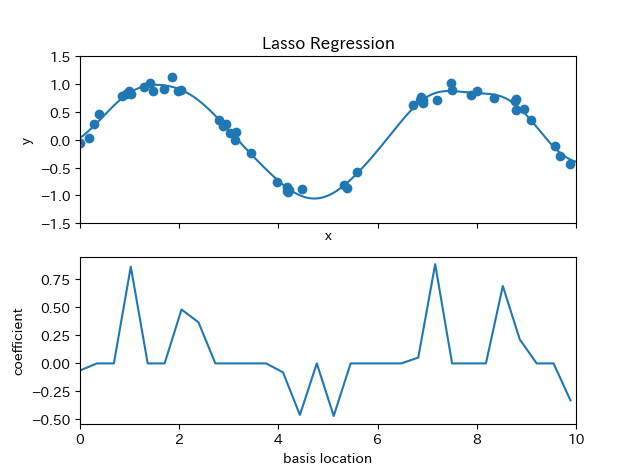
lasso更倾向于把系数设为0， 系数越高表示越过拟合